NASOS v4 - Results I cannot explain... (Patreon)

The first strategy of which I cannot explain its trading results.

Introduction

Hello my dear Patrons and welcome to another analysis of a trading algorithm in this Patreon exclusive post.

is time I tested multiple strategies that are called NASOS. There can be many versions found on Github and during my initial backtests the version 4 is the number performed the best on my backtesting setup. 

However there is something strange happening with this algoritm that I simply cannot explain for the first time I do all these tests.

Let’s first show you the source of this file and how it’s build…

Where to find it

As many other trading algorithms, this strategy is available on GitHub. If you search for the NASOSv4 file, then you will probably find lots of repositories that contain this file.

https://github.com/search?q=nasosv4&type=code

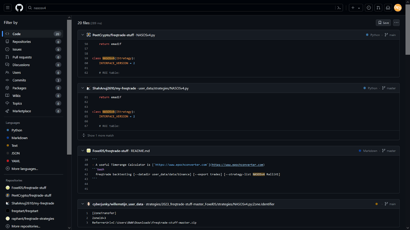
Let’s open the file and admire its contents…

The strategy

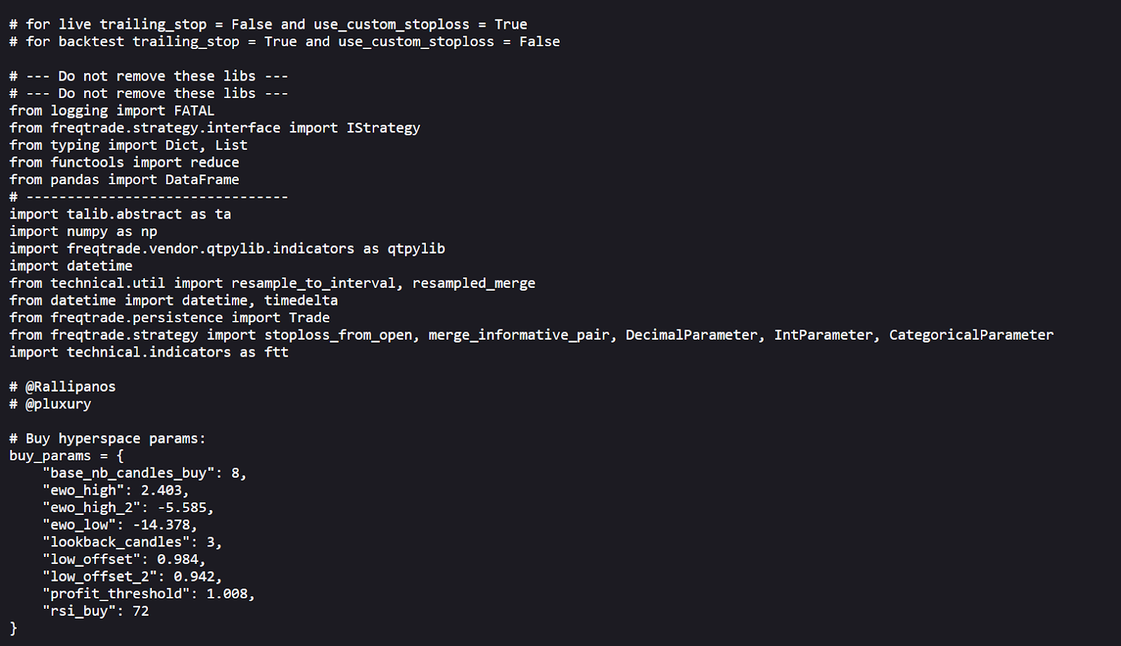
At the top of the file we can already find the first warning. You should set the trailing stop and custom stop loss parameters to true when live trading. And set the custom stop loss function to false when backtesting.

I will backtest this original file as it is here initially and then do a second test with the TSL disabled. 

In this file the custom stop loss is already set to false here.

A coder called Rallipanos made this algorithm and someone called pluxury also dit something with the code. It’s not my code, im just testing it to see if it is worthwhile for further investigation and maybe live trading. The trading idea and workings come from these great minds and I am just reverse engineering what they had in mind with this algorithm.

So let’s continue…

The first section shows us the hyperspace parameters, so we already know we can set multiple indicators to optimize this strategy. However, I will not do this since my last experiences are that further optimization only worsens the performance.

Then we have the well-know Elliot oscillator, that seems to be present and used in most of the well performing strategies. 

And after that the ROI table and Stop loss. Which has currently been set to sell at 15 percent loss if a trade goes bad.

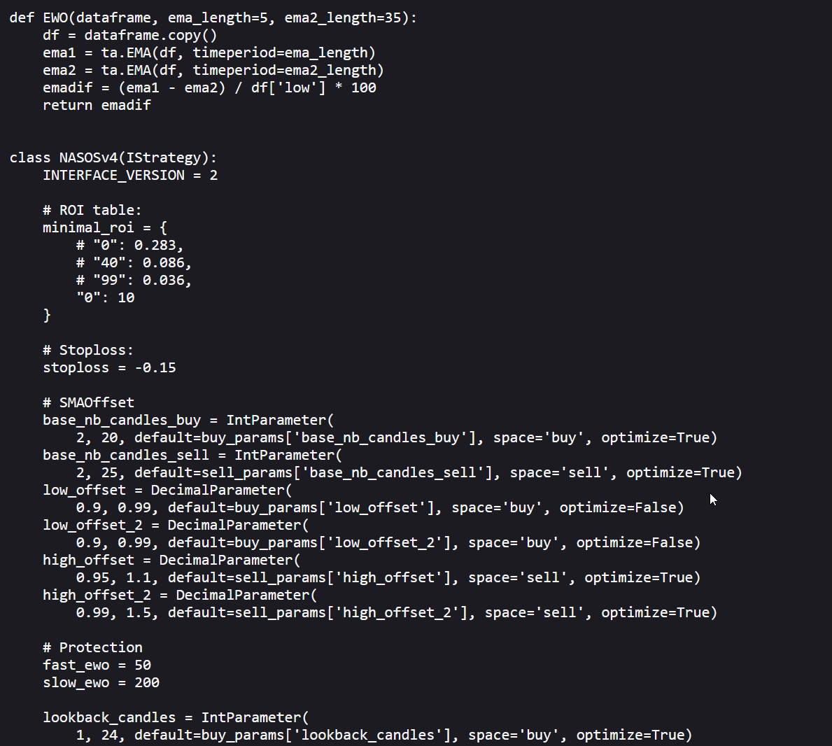
Then we have some more hyperparameters to optimize for the indicators that are used in this strategy

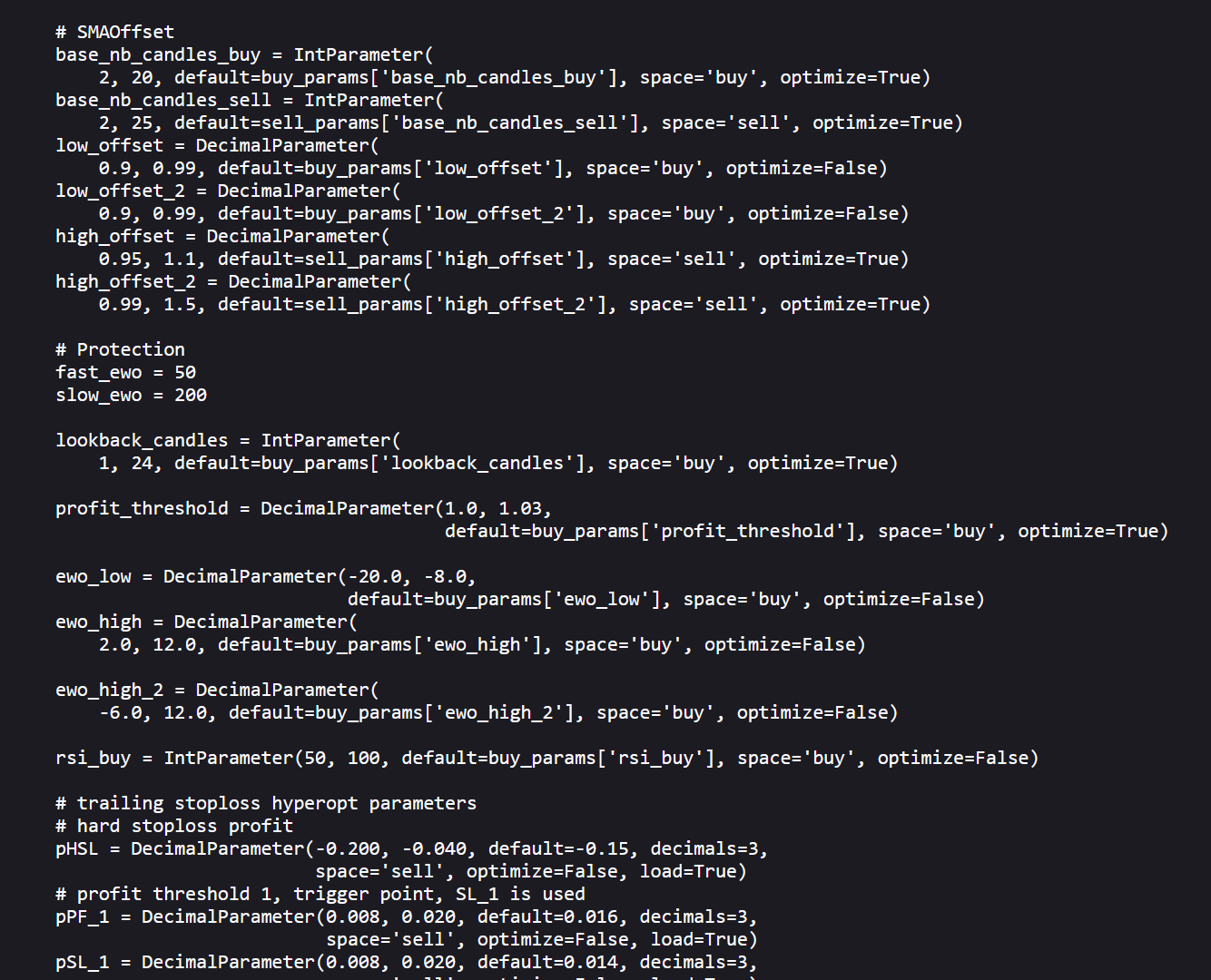
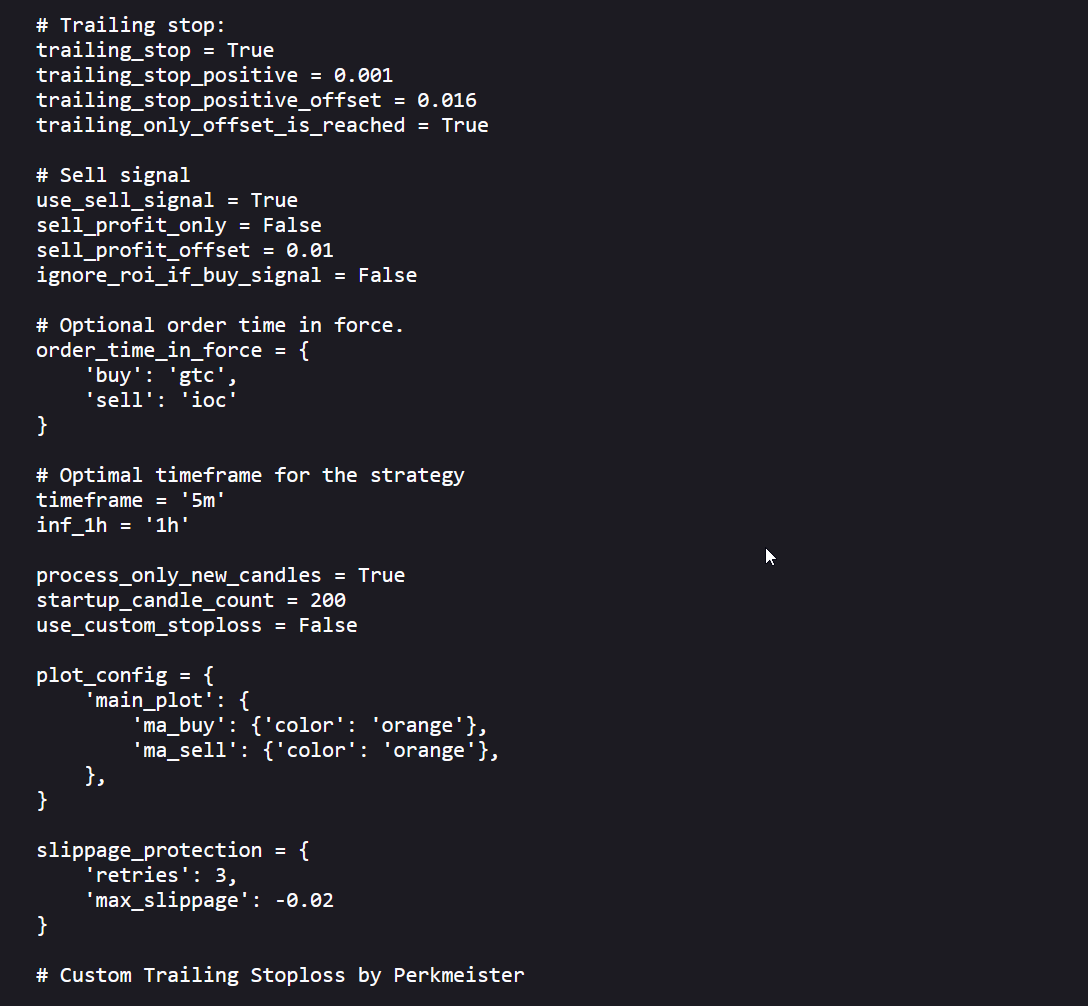
And then there are the trailing stop loss settings and the time frame that indicates that this algo has been built for the 5 minute timeframe.

After this we discover some interesting methods.

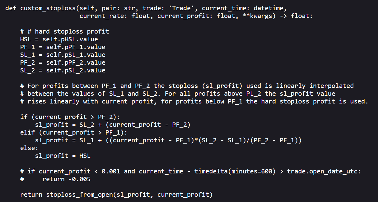
The first one is the custom stop loss, that has been disabled by default. But Lets run over it anyway…

This custom stop loss method in the strategy dynamically adjusts the stop loss level based on the current profit of the trade. If the profit exceeds a second, higher threshold, the method uses a fixed stop loss plus any additional profit beyond this threshold. 

Between two profit thresholds, it linearly interpolates the stop loss value. And below the lower threshold, it enforces a hard stop loss level. So this method aims to protect gains while allowing some room for price fluctuation, especially when profits are higher.

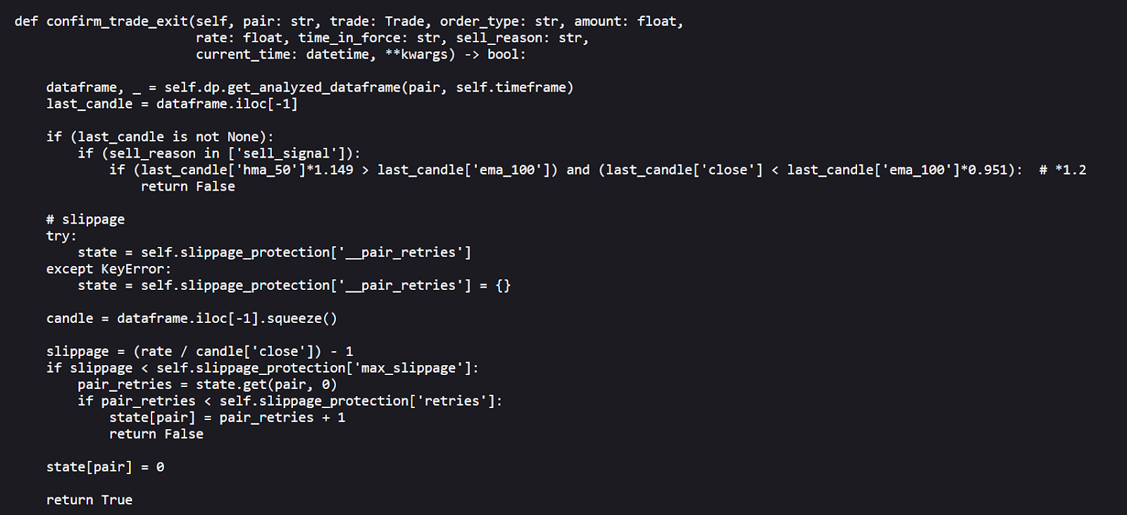
This confirm_trade_exit function in the strategy evaluates additional conditions to confirm or prevent a trade’s exit based on the last candle's data. It checks for specific price conditions against moving averages, like the hma and ema and tries to manages slippage by limiting the number of retries if the exit price is worse than expected.

Next we have the informative_1h_indicators function . This function is designed to fetch and potentially calculate additional indicators from a higher, 1-hour timeframe to inform decisions made on the primary trading timeframe. But as far as I can tell it seems to be a placeholder code, because almost all these calculations are commented out. 

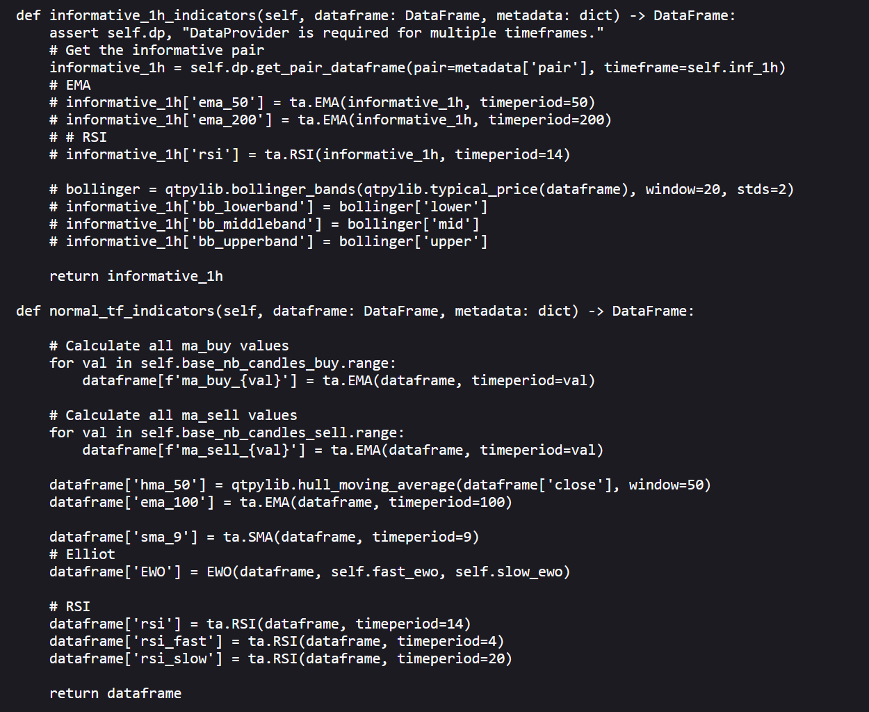
Now this normal_tf_indicators function computes various technical indicators for the primary trading timeframe. It calculates exponential moving averages (EMAs) for different numbers of candles specified in the buy and sell parameters, a Hull moving average, and multiple RSI values to track short and long-term momentum and trend directions within the trading strategy.

And the populate_indicators method orchestrates the incorporation of technical indicators into the trading strategy by merging the higher timeframe (1-hour) indicators from informative_1h_indicators with the primary timeframe indicators computed in normal_tf_indicators. 

So that I think the purpose here is that it first gathers any relevant higher timeframe data to enrich the strategy's context. And after that it applies the primary timeframe calculations to provide a comprehensive set of indicators. And this all is used to drive buy and sell decisions within the strategy. 

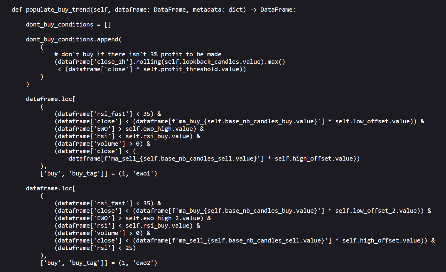
The populate_buy_trend method in the strategy defines the conditions under which a buy signal is generated. 

You can see that it evaluates multiple technical indicators like RSI and EWO values, alongside specific price conditions relative to moving averages, to determine suitable entry points. 

There are different conditions defined for different trading scenarios, and each of these scenarios is tagged distinctly (e.g., 'ewo1', 'ewo2', 'ewolow'). If you take a look at the output of the backtest, then you will see these buy reasons back. So you also have information which buy conditions occur most or have the highest profits.

Additionally, there's a dynamic check to avoid buying if the potential profit, as defined by a threshold relative to recent price highs, is not met. That method ensures that all specified conditions are met before signaling a buy, with additional provisions to cancel signals under certain situations through a series of "don't buy" conditions.

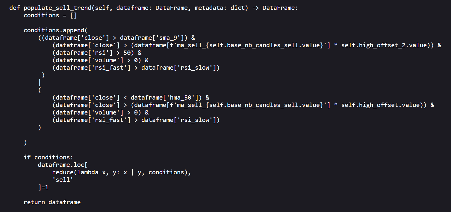
Now finally there is the populate_sell_trend method .

This method outlines the conditions under which a sell signal is triggered in the strategy. It uses a combination of price conditions relative to specific moving averages, RSI values, and volume to identify potential exit points. 

Also in this case, conditions are grouped to capture scenarios where the price exceeds certain thresholds or when fast and slow RSI readings indicate a change in momentum, that might suggest a sell. Only when one or more predefined scenarios are satisfied the open position in question will be closed. 

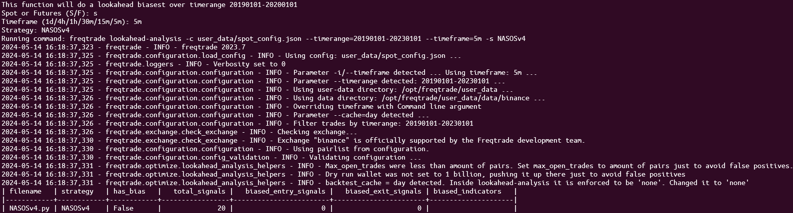
Lookahead bias

Now before I continue I also checked this algorithm on possible lookahead bias. But the built in function could not detect any as you can see.

Also I will show you later the difference in performance with and without the trailing stoploss set. So you can also take this bias into consideration when you decide to use this algo.

Backtest results TSL version

At the end of last year I discovered, what I thought, was the best trading algorithm. And I could not imagine that I would find even better performing trading strategies for my trading bot.

But as with many things in life, you can get pleasantly surprised. 

And with the results of this trading strategy, the limits are again stretched beyond my expectations.

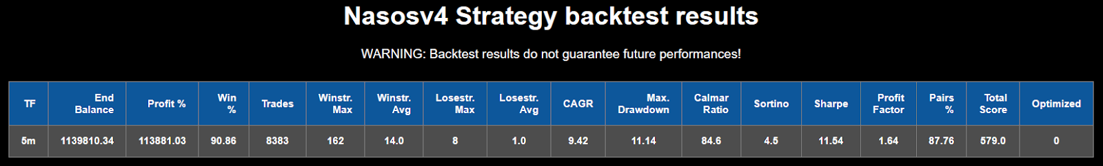
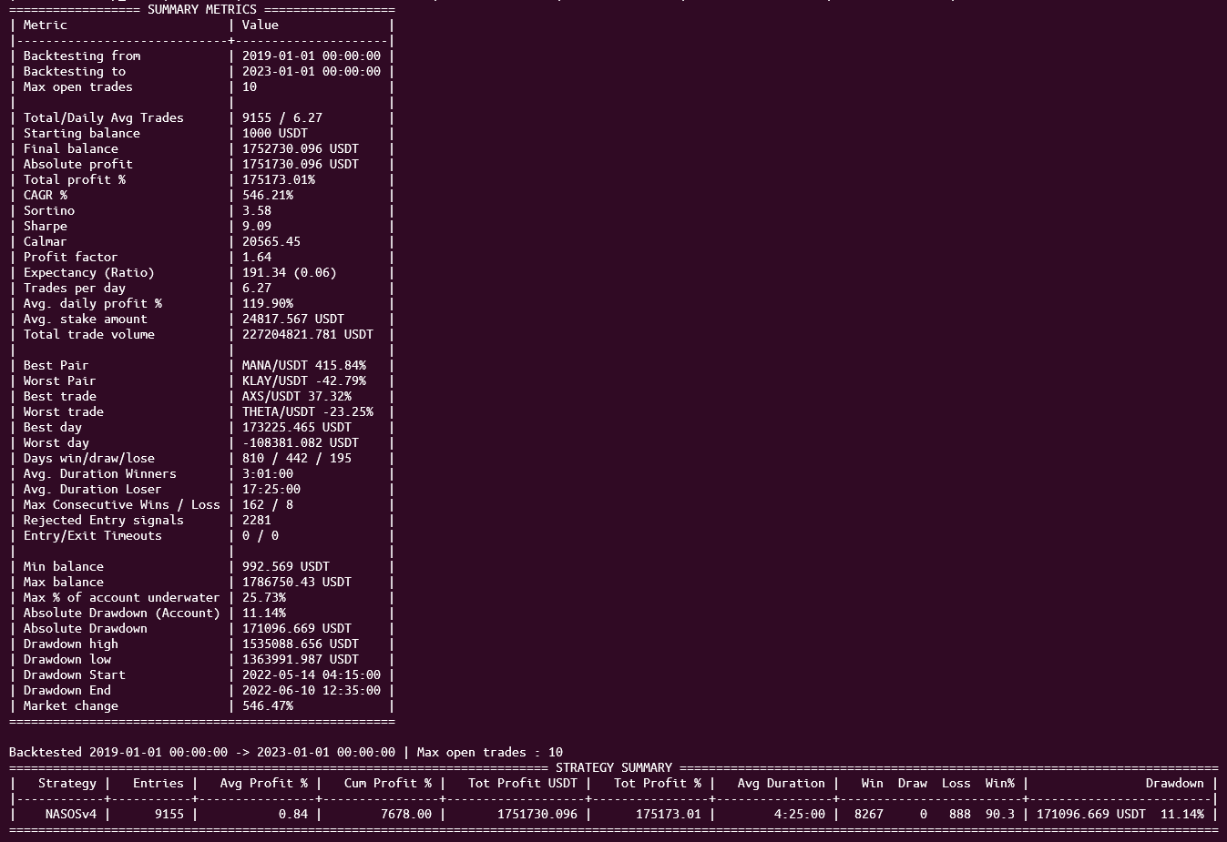
This trading strategy shows extremely good hypothetical trading results. 

Just like the MacheteV8b, this algo could trade over 1.1 million hypothetical dollars together. 

It has an over 90 percent win rate and max drawdown of 11 percent. 

87 percent of the pairs I use seem to get positive results with this algorithm.

Only a Calmar ratio of 84 looks to be suspicious to me. But let’s not let that spoil the fun.

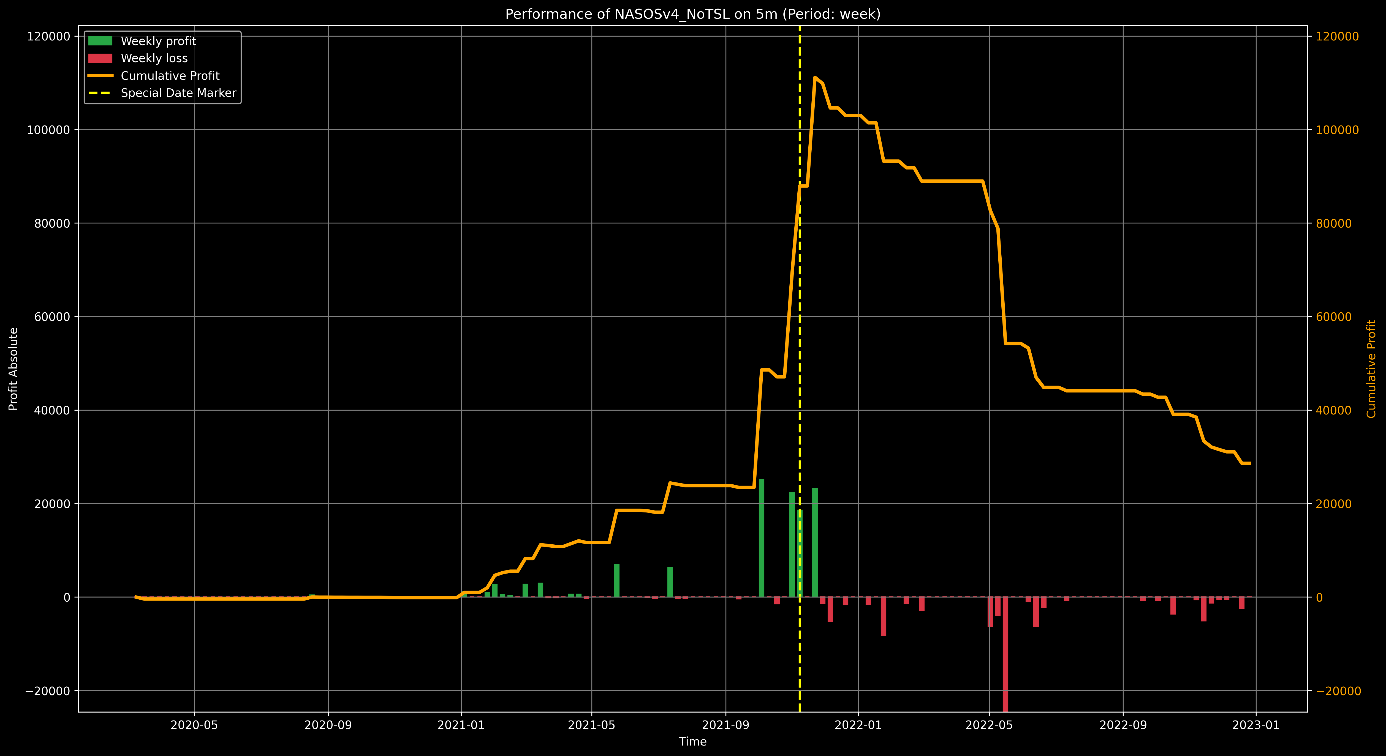
Let’s see how the equity curve looks like…

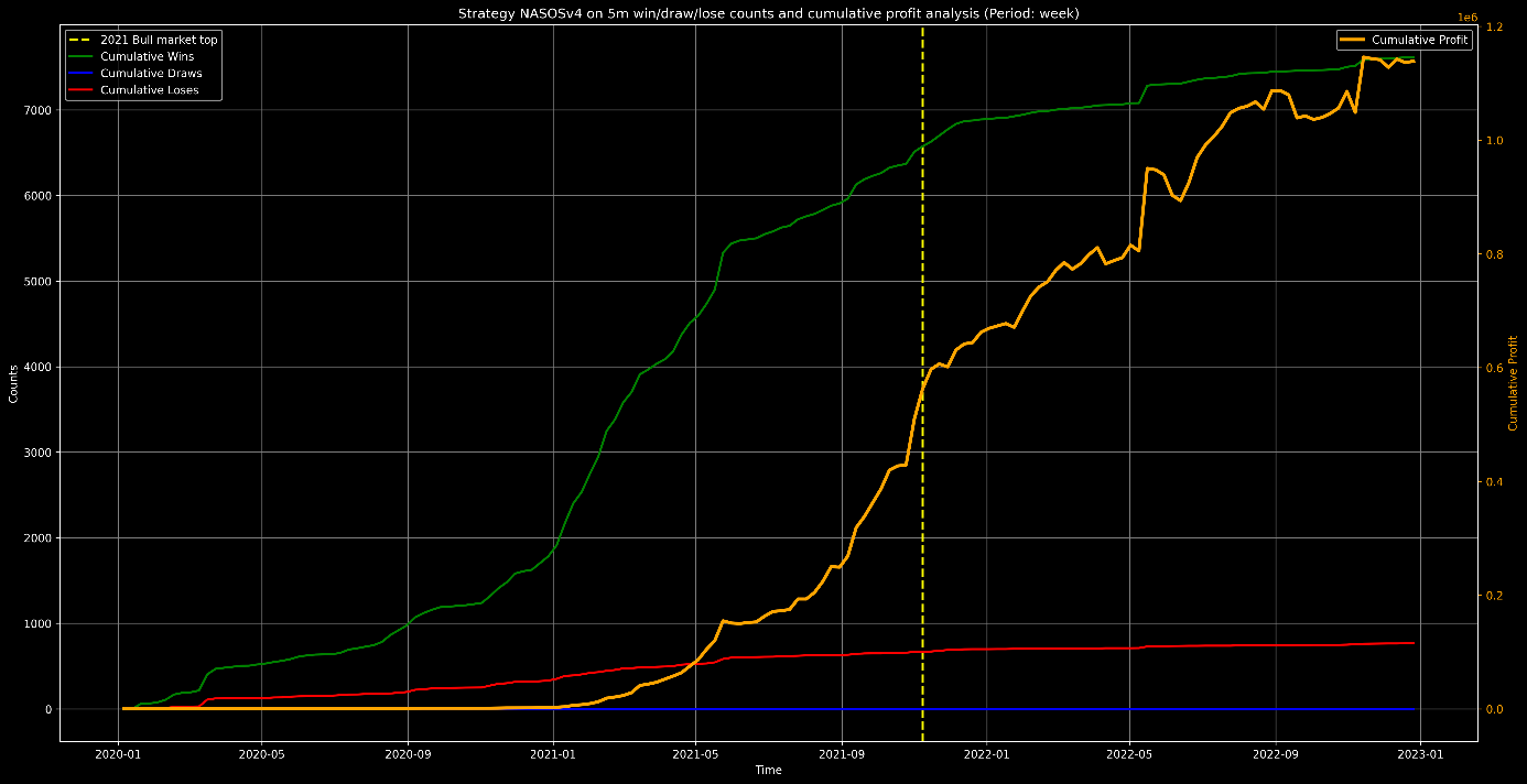
The over 1.1 million USDT has been reached by means of this journey of the equity curve. 

What’s so special is that after the previous bull market top, there is almost no decline. The curve and the wins keep on going.

The drawdown profile over the plotted timeperiod looks like this:

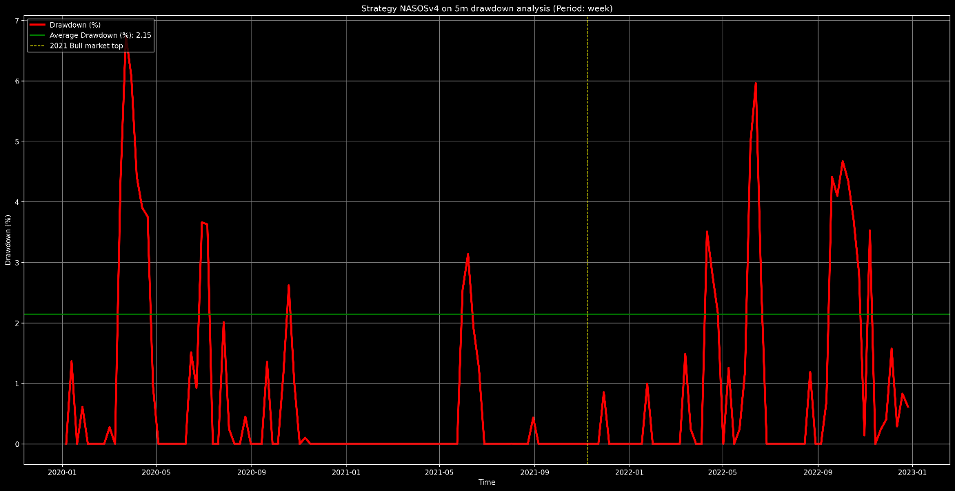
Some peaks around 6 percent drawdown and an average drawdown of a very admirable 2 percent. Note that the 11 percent drawdown in the table has occurred before the plots timeperiod.

The mean profit /loss over the complete backtest shows that it’s mostly positive. Only around the end of 2022 it gets negative. 

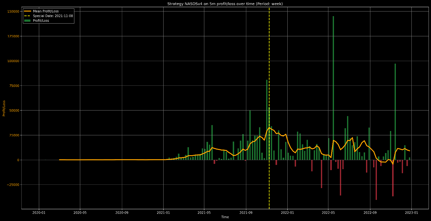
Also some weeks show very good profits. Like the week where almost 150.000 dollar has been traded. Now ofcourse there are also negative weeks, but these are manageable, although losses of over 25000 dollar would be a lot of pain. No matter how what happened before. 

Furthermore, the win rate distribution and profit distribution box plots are as follows.

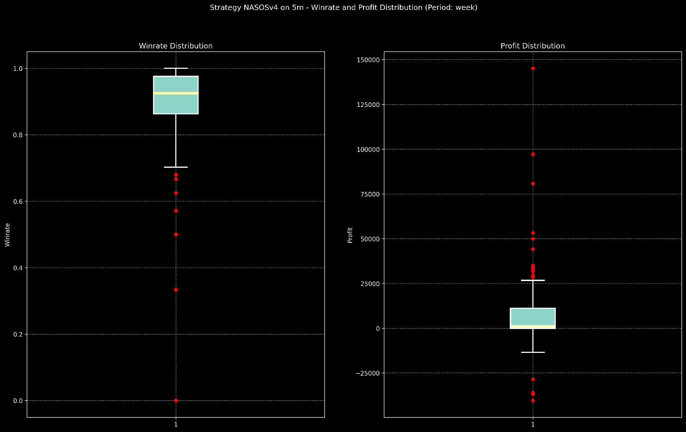
The box plot on the left shows a high median winrate, just below 1.0, suggesting that the strategy frequently wins a majority of its trades.

The interquartile range (IQR) is very compact, spanning from around 0.9 to just below 1.0.  And this indicates a consistent performance in terms of winrate.

Now, there are several outliers below the box. And these indicate weeks where the winrate significantly dropped below the typical range. That is also what we saw in the previous plot.

The profit distribution boxplot shows a wider range of values compared to the winrate distribution. And these profits vary significantly from week to week.

The IQR is centered around a median close to zero, suggesting that in many weeks the strategy neither makes nor loses a significant amount of money.

The outliers in this plot indicate that there are weeks where the profit is exceptionally high, as much as around 150,000, as well as weeks where the strategy incurs losses, around -25,000. 

All of this ends up in an indicator overview that looks like this:

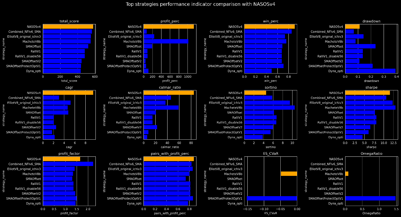
The colum is the highest or almost the highest where it should be high. Like win percentage sharpe, calmar and cagr. 

And the lowest or one of the lowest where it should be low. Like the drawdown.

This all results in a profit comparison plot between the top 10 best performing strategies that looks like this:

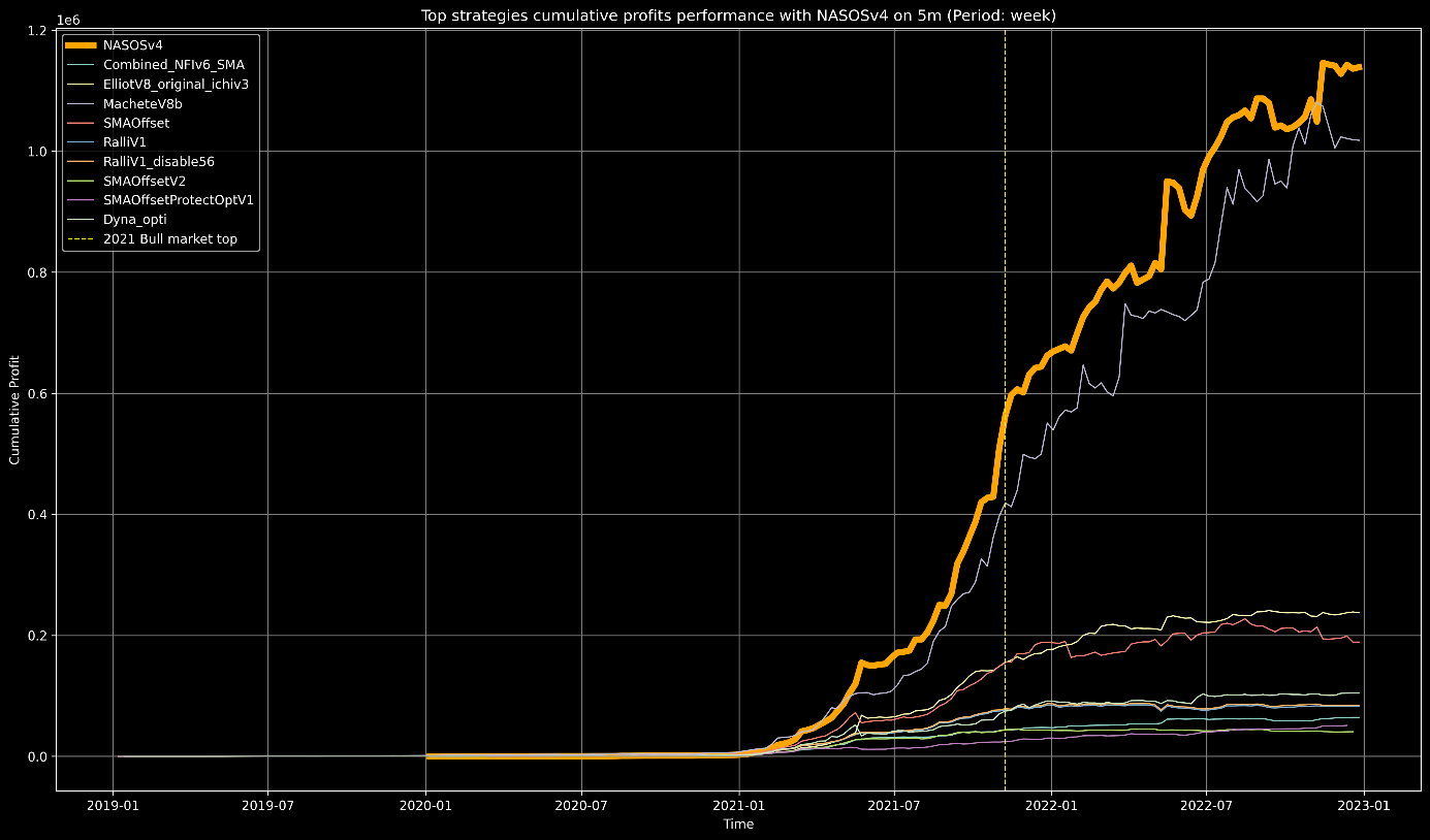
Where the NASOS performs the best of all. Even better than the MacheteV8b results.

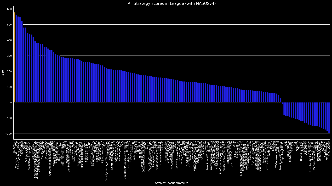
And you already guessed it ofcourse. With these results, this trading algorithm ends up at the top spot of the Strategy League.

A worthy position of this trading algorithm with its spectacular results.

Backtest results NoTSL version

But here comes the strange and unexpected part. 

Sometimes life can also throw you a curveball and you cannot explain why this happens...

:-\

As you might already know, I’m not a great fan of the Trailing stop loss function in backtesting. Since it can add a positive bias to the trading results. Using TSL can make a strategy more favorable because of it’s biased positive results. 

It could very well be that these positive results will not occur in real trading.

So I also tested this trading strategy without the TSL enabled and it got the following SHOCKING results back…

With a devastating equity curve.

To verify this difference I did a second test on another dataset and other pairs. 

On two machines with each their own setup. 

Machine 1

Machine 2

Now what on earth is going on here????

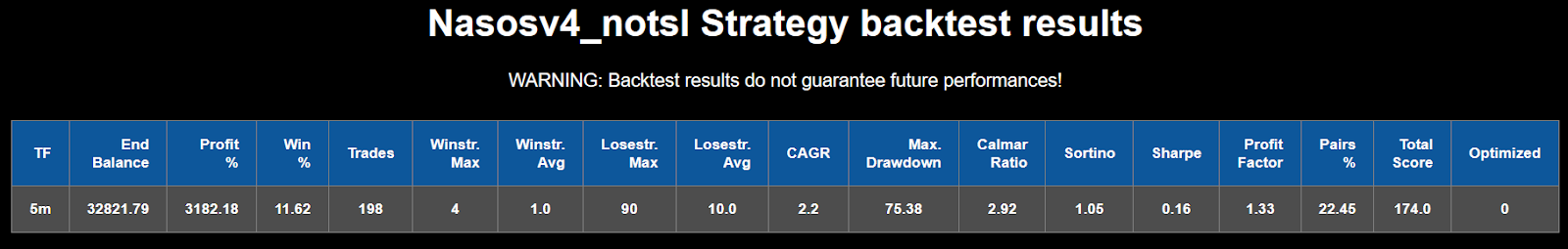
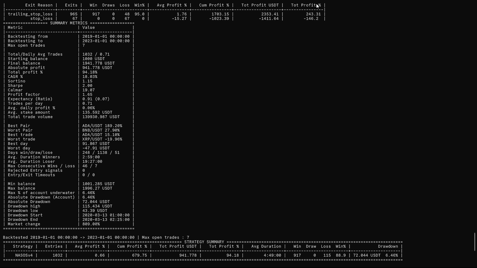
Again the backtest results between the TSL and NoTSL versions are these:

How can the disablement of a trailing stop loss setting give such a large difference in this particular trading algorithm?

Also, look at the amount of trades here…

8383 trades with TSL enabled and 198 with TSL disabled. 

How come? 

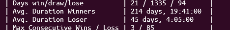
Well one thing that shows in the other individual tests is that with the TSL enabled, the average duration of winners is 3 hours and losers have duration of around 17:25 hours.

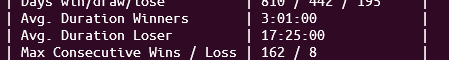
But with TSL disabled these numbers suddenly change significantly. 

214 days duration for winners and 45 days for losers. Why this sudden difference here??

If you see this colordiff here, then only these lines are different between the files:

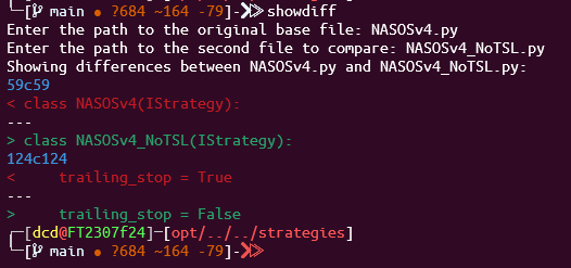
The secret may be in the first two lines of this code:

Here Backtesting should have trailing stop = True and custom stop loss = False

But in live trading it should be the reverse…

Unfortunately the Freqtrade documentation (https://www.freqtrade.io/en/latest/stoploss/#trailing-stop-loss) does not warn about the usage of trailing stops in backtesting. 

Also there’s nothing that the custom stop loss says (https://www.freqtrade.io/en/2021.2/strategy-advanced/#trailing-stoploss-with-positive-offset) about the difference in results between backtesting and live (forward) testing.

There is also no real  explanation found in the ‘Assumptions’ documentation section(https://www.freqtrade.io/en/2021.2/strategy-advanced/#trailing-stoploss-with-positive-offset). 

Except that:
Trailing stoploss

• High happens first - adjusting stoploss

• Low uses the adjusted stoploss (so sells with large high-low difference are backtested correctly)

• ROI applies before trailing-stop, ensuring profits are "top-capped" at ROI if both ROI and trailing stop applies

But this still does not explain to me why there are such big differences here. So this remains a total mystery to me. Maybe somebody else can explain what’s going on here..?

For me now the only way to check to see if this a valid strategy or not, is to add it to my forward testing trading bot to see what the actual performances will be under ‘live’ conditions.

For now I will leave the results in my strategy league for what they are and if forward testing shows that this strategy is really bad, then I’ll remove the results. So not to misinform other people in the future.

Ending

So with this exceptinal conclusion I am at the end of this post. 

Again, maybe somebody can explain this large difference if he/she tests this on their own setup. And if you did, then please add your findings to the comments section of this post.

This is it for me now, and I will see you in the next post.

Goodbye!